College Football Recruiting Maps & Analyses - Summary
To rehash my intro paragraphs from the home page:
One way to quantify a college football program's potential for success is to assess its probability of drawing in top recruits. Much of recruiting potential is dictated by the coaching staff and a school's prestige but geography plays a large role as well. The easiest way to observe this effect is to check out any team's roster. Both public and private schools will fill the bulk of their roster from students within a few hundred mile radius (e.g. 50% of players live within 250 miles of their school; see more details in "Methods" section).
Therefore a school's recruiting pool can be quantified by the population of the surrounding areas; in other words if we know how far away recruits are willing to travel, an effective population can be calculated for any location in the country (if you know the point sources of all populations). It's also important to look at the effect of schools competing for recruits, that is a school might have access to many recruits but these recruits might have offers from other nearby colleges. In this way schools were treated as negative populations.
In this way the 120 Division I-A schools can be ranked by their effective populations and places without schools can also be shown to be ideal places for a new program to crop up (theoretically). Schools can be also be shown to be over or underperformers.
How to account for the effect of geography (distance from recruit to college)
The first step is to figure out how geography plays a role. To do this I took the 120 Div. I-A rosters from 2009 and calculated the distance from each player to their school. Taking it in 50 mile increments, I was able to fit a function to describe this relationship for ANY distance up to 2000 miles:
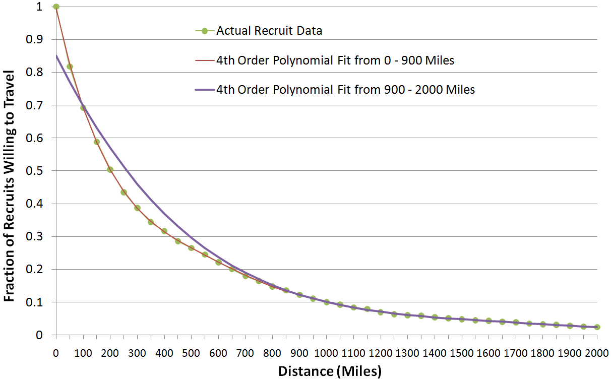
What this graphs says is that ~80% of recruits live more than 50 miles from their school and ~4% live more than 2000 miles away. This data can also be interpreted as saying, 20% of recruits are willing to travel no more than 50 miles and 96% of recruits unwilling to travel more than 2000 miles to go to college. See here for more.
Two approaches to modeling the data
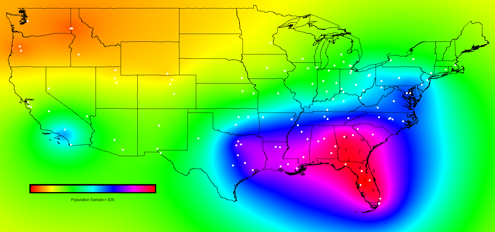
With those numbers in mind, if we locate a recruit in Tampa, Florida, he's ~80% willing to go to a school like Miami, but only ~5% likely to choose a school like UCLA. We can add in recruits from across the country in this fashion and we can say given a recruit at location X, he's Y% willing to go to a school at location Z. We can do this for any spot in the US and generate a nice-looking map showing where the "effective recruiting potential" is highest. This "effective recruiting potential" indicates how many recruits a school is liable to have access too (i.e. the sum total of all recruits times their willingness to go to a particular location). We can also consider the effect of competing schools in the vicinity by considering them "negative recruit populations" that reduce the recruiting potential of nearby schools.
The second way to approach the data is what I call the "normalized probability" method. In this instance I'm only looking at recruits going to a certain school (not any location Z on the map). I can say, based on geography, this recuit is 80% willing to go to Miami, but he's also 75% willing to go to Florida State. I sum these per-school probabilities and then normalize them to one (i.e. recruit chooses one school only). Each recruit contributes some probability to all 120 schools based on their geography (and other testable factors).
Scaling the recruiting potential
Geography of course isn't the only factor in how a recruit chooses a college. One easy way to discern between teams is whether they are big time programs. Any easy was to draw this line by whether or not they play in one of the "Big 6" conferences (ACC, Big East, Big XII, Big Ten, PAC-10, SEC). So the probability of a recruit choosing one of the non-Big 6 teams is less and theses schools are less able to steal away recruits from their neighbors. Another important factor is winning percentage, both recent and historical. A recruit wants to choose a school that has won lately and has a high prestige factor. In this way, winning begets winning, but looking at the data it is certainly an important point to consider. These various scaling factors are included in the "sub-analyses" linked to on the home page.
Who is a recruit?
These are what I call my "population sources". In other words who are schools trying to recruit? Are they looking for large populations like New York City?--for this I use the 2000 US Census (Case 1). Are they looking for the elite players?--for this I've used the last four years of the Rivals 250 list (Case 3). Another way is to go back to the players already playing (about 12,000 of them on the 120 I-A rosters) and assume they do a pretty good job of identifying where future recruits are located (Case 2). It's interesting to note that the actual population does not at all mirror the population of people who are good at football.
What does this all mean?
Still working on this! The maps tell you the best places to recruit. If you're a coach and looking for your next job you might want to pick a school with a high "effective recruiting population" that has been underperforming. This pretty much means the southeast corridor from Florida west to eastern Texas. You can also ask, who has a tough job?--That would be coaches in the Pacific northwest.
The "normalized probability" method is great at seeing who recruits poorly because if gives you real, expected values for teams. You can see, for instance that Georgia Tech, in Atlanta, is the best place to recruit, but they typically underperform. You can see the top programs of the decade are cleaning up when it comes to aquiring the top recruits (which helps them win more). But by minimizing the error in the predictions versus the actual results by adjusting various scaling factors you can see how much different variables matter in recruiting. There will be much more to come!
Please let me know your thoughts, insights, questions, comments, etc: tbrennan "at" stanford.edu